Read the Room:
A Small Transformer Learns to Bet on Cricket Fights

Michael Siu · Jul 27, 2026 · ~15 min read

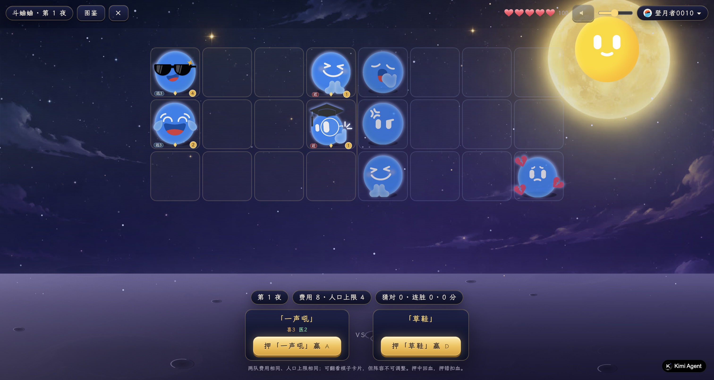
There's a little auto-battler¹1Auto-battler: a genre where you draft and position a team of pieces, then watch them fight automatically — no micromanagement, the draft is the gameplay. Think TFT or Auto Chess. called Moon Mood Tactics (月面情绪棋, "moon-phase emotion chess") on k399.games, a new project here at Kimi demoing AI-built games. Every piece in it is an emoji with a mood, and synergies are literal moods: 喜怒哀静 (joy 喜, rage 怒, sorrow 哀, calm 静). It has a PvE mode, a ghost-PvP mode, and, the star of this post, a mode called 斗蛐蛐, cricket fighting.

Cricket mode works like this: every night, the game presents two teams with identical total cost and identical population cap, mirrored across the board. You can inspect every piece, but you can't touch anything. You just bet: A or B. Right bet heals 5 HP; wrong bet costs you 6 plus the star-sum of the winner's survivors²2The penalty mirrors the standard mode's loss formula. Getting stomped hurts more than edging a loss: surviving 3★ units add up fast. (getting stomped hurts more). HP hits zero, run ends. Blind betting survives about 22 nights on average, by design. The mode was meant to reward people who can read a team composition.

I got annoyed at my own win rate and decided to make it a weekend project: solve this mode with a model. A week later, a run driven by a 318k-parameter transformer had survived 584 nights and taken the leaderboard's #1 spot. Here's how. And here's the one rule I set for myself: the model only ever sees what a human sees, namely the two team layouts. More on that rule in a moment, because it's the whole premise.

#1The five-minute realization

Three facts about our own game made this project almost unfairly convenient:

• The battle simulation is fully deterministic. A night's layout is derived from (gameSeed, night), and the battle RNG from a fixed XOR formula.³3Seed contract: cricketSeedFor = seed ^ night·0x9e3779b1, battleSeedFor = seed ^ night·0x85ebca77. Same inputs, same outcome; that's also how the daily mode stays fair. Same inputs, same outcome, every time.
• The whole engine is pure ESM JavaScript with zero DOM dependencies. You can node simulate.js a battle in ~0.3ms.⁴4~0.3ms per battle, single-threaded. A million labeled samples costs a lunch break, not a compute budget. No scraping, no reverse engineering: just import the game's own code and run it a million times.
• Betting doesn't change the future. Night layouts depend only on the seed, not on your choices. So there's no credit assignment, no exploration, no RL loop. Each night is an independent question: given these two teams, what is P(A wins)?

But wait: if the simulator is deterministic and I know the seed formulas, can't I just compute the winner? Yes. And no, that's not the experiment. Exact replay would trivially solve the leaderboard, and teach nothing. So I drew an information boundary on purpose: the model sees only the two team layouts, the same information a human player gets. The seed is used only to materialize those visible layouts; neither gameSeed nor the battle seed enters the model input. The exact simulator runs alongside it purely as a shadow oracle: it never informs a bet, it only checks afterward that the online game still matches my local engine bit-for-bit (more on that in §5).

One subtlety inside that boundary: the battle seed is hidden from the player, and battles contain genuine randomness (random skill targets, proc chances). The same matchup can go either way. So the right target isn't a 0/1 label, it's a probability, estimated by Monte Carlo. Say lineup A beats B in 6 of 8 simulations: calling it "A wins" throws away the most useful information: it's a 75/25 matchup, not a certainty. The label is the win rate over K=8 battle seeds,

$$\hat{y} \;=\; \frac{1}{K} \sum_{k=1}^{K} \mathbf{1}\big[\text{A wins under battle seed } k\big]$$

and the loss is plain binary cross-entropy, which has a lovely property when the labels are probabilities:⁵5Why K=8: cheap and good enough for decided games, which dominate. The label noise that remains lives in the genuinely-close matchups, exactly where the model should be unsure anyway.

$$\mathcal{L} = -\big[\hat{y} \log p + (1-\hat{y}) \log(1-p)\big]$$

$$\arg\min_p \, \mathbb{E}[\mathcal{L} \mid x] \;=\; \mathbb{E}[\hat{y} \mid x] \;=\; P(\text{A wins} \mid x)$$

In words: the model is rewarded for saying 0.7 on matchups that A wins 70% of the time, not for pretending every matchup is certain. That's the win-rate function we are asking it to learn, rather than a collection of hard outcome labels.

Before training anything, I measured the ceiling: 1,500 random layouts, 16 battle seeds each.

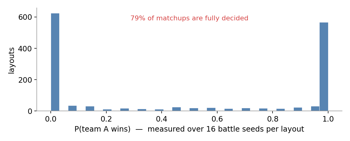
So the task: learn a function from "two team layouts" to "P(A wins)", with an estimated ceiling around 95% and a coin-flip floor at 50%.

#2Manufacturing a dataset

The pipeline, end to end: sample a random seed and a night, build both teams with the game's own team builder, simulate the battle 8 times with different battle seeds for the soft label. Each sample is one night's two teams, flattened into 377 floats:

sample (377 floats)
├── globals: night, popCap, budget
└── per team ×2 (A left, B right)
    ├── 55 aggregate stats: hp, dps, trait levels, per-unit star sums…
    └── 12 unit slots × 11 fields: identity, star, x, y, cost,
        effective hp, dps, mana, range, ability

A million labeled examples for the price of leaving a Node process running over lunch. No annotation party required. The game grades its own homework.

#3The model ladder

I trained four candidates on the same sampled layouts and splits (each model family gets its own featurization, which is part of the architecture, as we'll see):

Version names, since they'll keep coming up: v1 = a 100k-sample pilot dataset; v2 = 1M samples, nights 1–44, used for everything in this section; v3 = the same million samples but with nights redistributed to match real play. More on why that mattered in §5.

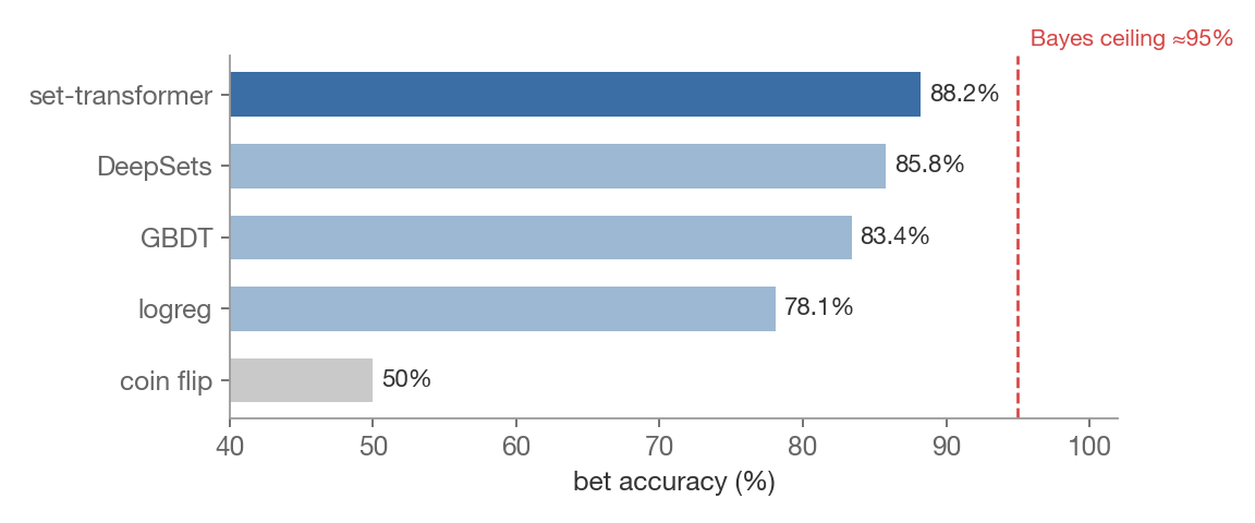
The interesting part isn't the ranking, it's why. A tiny example of the core issue: an assassin isn't inherently strong, and a backliner isn't inherently weak. But put "my assassin" and "your exposed backliner" in the same game and the win rate swings. A linear model can only write

$$z = w_1 \cdot (\text{assassin}) + w_2 \cdot (\text{backliner}) + \dots$$

when what the game actually rewards is the product:

$$z = \dots + w_{12} \cdot (\text{assassin} \times \text{exposed backliner})$$

• Logistic regression (78%) is stuck at the first equation: total HP diff, total DPS diff, everything additive. It structurally can't say "counter".
• GBDT (83%) can build exactly those interaction terms out of thresholds, but only over hand-aggregated features, where positioning information already died in the compression.⁶6LightGBM vs sklearn's HistGBM: identical accuracy (82.8%), 2× faster fit. The library isn't the lever; the features are.
• DeepSets (86%) eats raw unit sets, but teammates never see the enemy until the final layer.
• Set-transformer (88%) lets every unit attend to every unit on both teams from layer one, so an assassin's representation is computed in the context of your squishy backliner standing in the corner. More on why this works in the next section.

One more honest data point: at 100k samples the transformer and GBDT were tied (~83%). At 1M samples the transformer gained 5.3 points from the extra data while GBDT gained 1.⁷7Scaling check: GBDT 82.4→83.4, DeepSets 82.2→85.8, transformer 82.9→88.2 going from 100k to 1M samples. The architecture gap only shows up when the data can pay for it.

#4Why attention fits (a hypothesis)

Why should attention be the right inductive bias here? Two structural properties of the problem point at it.

First, the input is two unordered sets. A team is a set $S = \{u_1, \dots, u_n\}$; permuting the listing order must not change the prediction, $f(\{u_1, u_2, \dots\}) = f(\{u_2, u_1, \dots\})$. (The units' $(x, y)$ board positions are properties of the unit and absolutely should matter; that's different from array order.) One symmetry is deliberately not imposed: swapping teams A and B is not neutral, because the rules themselves aren't symmetric (ties go to B, placement is mirrored), and A wins about 53% of otherwise mirror-fair matchups.⁸8Design consequence: one shared encoder for both teams, no positional encoding, side identity kept as an input. The invariances are built in, not learned from data.

Second, the interaction term needs a home. DeepSets compresses each team first ($\operatorname{pool}_i \varphi(u_i^A)$, $\operatorname{pool}_j \varphi(u_j^B)$) and only then lets the two meet, so matchup-specific pairwise structure has to pass through fixed-size pooled summaries. Joint attention lets every unit build its representation in the context of the specific opponents it faces:

At one attention layer, every unit token starts as a vector $x_i$ containing its current representation. From that vector, the model makes three learned views:

$$q_i = W_Q x_i, \qquad k_i = W_K x_i, \qquad v_i = W_V x_i$$

The simplest mental model is: queries and keys decide who should talk to whom; values decide what gets said. When updating unit $i$, the model treats $i$ as the receiver and lets $j$ range over every unit it could listen to:

• Query $q_i$: the receiver's search vector — “what kind of unit should affect me?”
• Key $k_j$: a candidate sender's matching vector — “am I the kind of unit you are looking for?”
• Value $v_j$: that sender's payload — “if I matter, this is the information I will pass to you.”

Keeping key and value separate is useful because the features that make a unit relevant need not be the same information worth importing from it. Suppose $i$ is an assassin and $j$ is a cornered enemy marksman. The assassin's query and the marksman's key may form a strong match because of side, role, and position; the marksman's value can then pass along whatever learned mix of stats, role, and position should change the assassin's representation.

The calculation follows that story from left to right: score how well each key matches the query, normalize those scores into weights, then mix the values using those weights:

$$s_{ij} = \frac{q_i^\top k_j}{\sqrt{d}}, \qquad \alpha_{ij} = \frac{e^{s_{ij}}}{\sum_\ell e^{s_{i\ell}}}, \qquad c_i = \sum_j \alpha_{ij} v_j$$⁹9In the actual model: four attention heads run this calculation in parallel, each with its own $W_Q$, $W_K$, and $W_V$. A residual connection and an MLP then turn the resulting context into the token's next state. The equation here shows one head.

So a strong query-key match gives the marksman a large weight $\alpha_{ij}$, and more of its value flows into the assassin's context vector $c_i$. The result is a summary of the lineup from this unit's point of view: not just “I am an assassin,” but “I am an assassin facing this particular exposed backliner.” The projections are learned end to end; those meanings are an intuition for the mechanism, not hand-coded features or a claim that one attention head must literally represent “backliner vulnerability.”

The 24×24 attention matrix gives the model a natural place to represent matchup-specific relationships, something resembling a soft, context-dependent counter table. Attention weights aren't a causal proof, but the +2.4 points over DeepSets, an architecture that differs mainly in where the teams are allowed to meet, is consistent with the mechanism mattering.

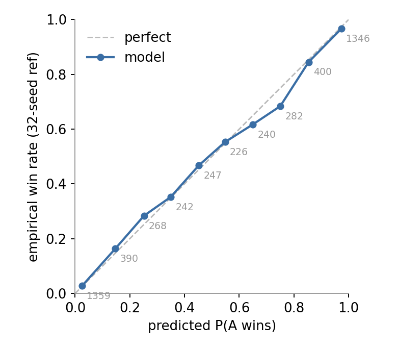
And the probabilities are real. The model's output drives actual bets, so it had better mean what it says. On 5,000 held-out layouts, predicted probabilities track the empirical win rate closely, a little overconfident in the 0.6–0.75 band, near-perfect at the extremes where most of the mass lives:

#5Into the wild: it worked, then it worked worse, then it worked

Playing for real required exactly one thing: the run's gameSeed, which the server helpfully returns from /api/cricket/run/current. With the seed, I compute every night's layout offline, run the model, and POST the bet through the game's own session.

As an integrity check, every night I also re-simulate the battle offline and compare against the server's verdict; a mismatch would mean the online version drifted from my local engine. Across thousands of bets: zero drift. Bit-exact.

The first live run survived 334 nights and put me at #1. But something was off: live accuracy was ~84% vs 88% on the test set. The culprit turned out to be my own sampling distribution:

Training nights were uniform 1–44. But the game's difficulty caps at night 44 (12 units, 180 budget), so a real long run spends ~85% of its nights in that "capped config", which was 2.3% of my training data. The model spent most of its live career slightly out of distribution.

v3 fixed it by sampling nights 1–200 (78% capped-config).¹⁰10Deployment-shaped eval: episode replay (official seed stream, capped-config dominated) is the only metric I trust for comparing versions. Survival went 135.5 → 140.1 nights.

#6Battle report

After one 71-night shakedown run (variance is real), nine automated live runs with the v3 model: 106 / 106 / 124 / 209 / 238 / 335 / 443 / 553 / 584 nights, median 238. The best run, pictured below, is now the leaderboard's top score.

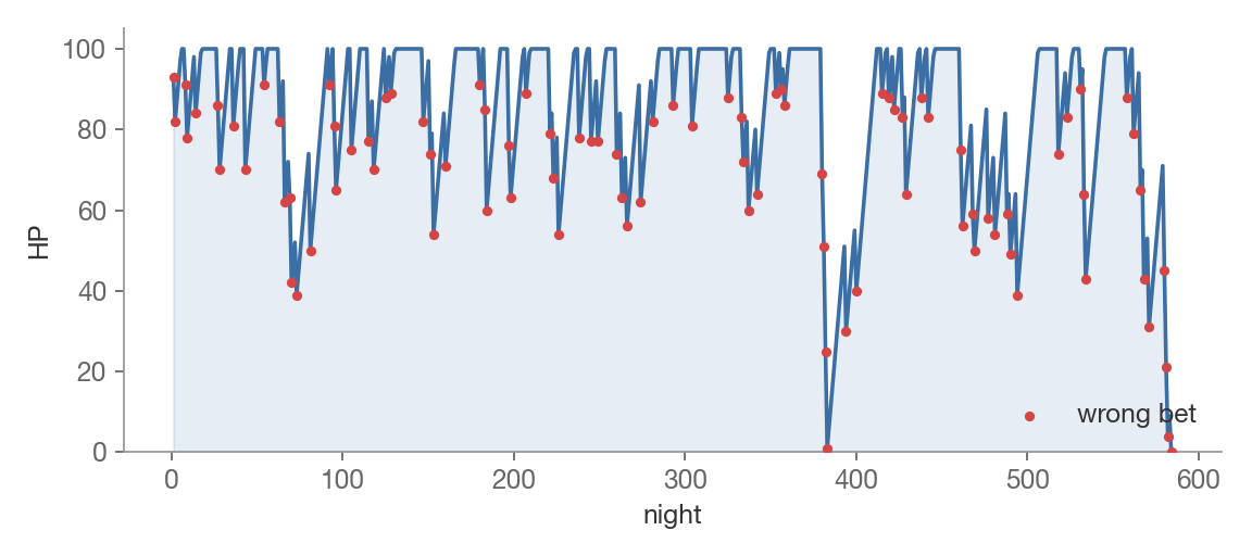
	best run	score	leaderboard
v2 model (first contact)	334 nights	4,097	#1
v3 model (after OOD fix)	584 nights	15,205	#1
blind betting (design baseline)	~22 nights	~230	—

There's a hard cap of 999 nights in the rules¹¹11MAX_NIGHT: 999 is defined in the shared rules but never referenced client-side; server-side enforcement unknown. We haven't reached it either way; every run died of variance first. I haven't reached it; every run so far died of variance first. Back-of-envelope: at ~85% accuracy the expected HP change per night is positive, so death requires a genuine losing streak, and long streaks get exponentially rarer as the HP buffer grows. The early nights, before the buffer builds up, are where runs go to die.

#7What's next

• Longer training, cleaner labels. The val curve was still creeping down at 40 epochs, and K=16 soft labels would make the genuinely close-matchup labels noticeably less noisy. Cheap wins, both.
• Ensemble. GBDT and the transformer are wrong on different matchups, so averaging their probabilities is a cheap experiment with a real chance of helping. It also pins down how much headroom is left before the ~95% ceiling.
• Betting for survival, not just for win rate. Pure argmax-P ignores that a wrong bet costs 6+variable survivor stars; at low HP, the low-variance side of a 50/50 is worth real survival probability. Whether that's best handled by a cost-sensitive classifier, a bit of dynamic programming, or a small RL fine-tune is an open experiment.

Cricket mode is a toy but honest testbed for a broader question: can a simulator turn a stochastic, set-structured combat system into a learnable matchup evaluator? Here, one small transformer learns a useful local answer — given two fixed teams, who is favored and by how much. A full TFT-playing agent would still need the harder layers: drafting, economy, positioning, opponent modeling, and long-horizon planning. This project solves only the matchup layer, but that is a real piece of the puzzle.

---

Views and experiments are my own. This is a personal side project.

The game: Moon Mood Tactics on k399.games, v2.5.1. All experiments run locally on a laptop; battles simulated with the game's own unmodified engine. Model: 318k-param set-input transformer, trained from scratch on 1M self-generated labeled layouts. The leaderboard is still open if you want to try.